
The files for this tutorial are available on github.com/ac2cz/SDR
It was a lot of fun creating our simple Direct Conversion SDR and listening to signals on the bands. But there are some serious drawbacks in our simple radio that need to be addressed. The most serious is our inability to select a sideband.
With I and Q we are able to determine the instantaneous amplitude and phase of our signal. That will allow us to demodulate AM and FM signals. Or PSK for that matter. Right back in Tutorial 1 we gave the calculation for the Magnitude and Phase of the FFT result. It is the same formula that we use for the Magnitude and Phase of our I/Q signal.
    mag = sqrt( I^2 + Q^2)
    phase = arctan (Q/I)
If we calculate the magnitude and use that as our audio then we will demodulate AM. We are recovering the shape of the audio envelope which was used to modulate the RF carrier. If we use the rate of change of our phase (not just the instantaneous phase) then we will demodulate FM.
Demodulating Single Sideband is a little trickier. I won't repeat the math here, because it is treated rigorously in Experimental Methods in RF Design by W7ZOI et al and in Understanding Digital Signal Processing by Richard Lyons. It is also discussed online in multiple places.
Remember the flow diagram for our SDR? I have added some boxes in red that will achieve our SSB demodulation. This is the so called "Phasing Method" of SSB demodulation. In my homebrew radio there is no need for "decimation" but the -90 degree phase shift is there and is achieved by op amps. When we sum the I and Q audio we get LSB or USB. If we swap I/Q (using a toggle switch of course) we change sidebands.
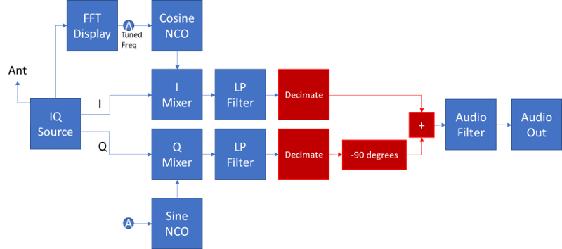
In our Software Defined Radio we will implement the -90 degree phase shift with a Hilbert Transform. We can then add the resulting audio to get LSB or subtract them to get USB. (Swapping I and Q as I did in hardware would have the same effect, but we don't need to do that.)
But before we do that, let's cover decimation because we want that working and tested first.
Any FIR filter requires a lot of multiplications and adds. Our Hilbert Transform will be no exception. We can dramatically reduce the load by reducing the bandwidth of our signal. Our SDR samples the data at 192000 samples per second, or perhaps more. If we reduce that bandwidth then we will have less calculations to do. As an experiment, let's try decimating to 48000 samples per second, because that is a good bandwidth to play out our speaker. We could decimate more, but decimation by 4 will illustrate the concept and reuse the filters that we already have.
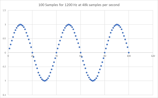
Decimation consists of two steps. Filtering and down-sampling. Down-sampling is easy. We just throw away the samples that we don't want. Really. Let's remember our waveform from Tutorial 1. It was 1200Hz at 48000 samples per second. If we go back to the code and generate the first 16 samples of the above and print them out, and then do the same for the first 4 samples with the sample rate changed to 12000 samples per second, then we get these values:
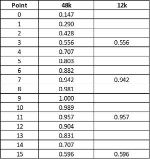
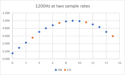
We know from Tutorial 1 and from our discussion of the Nyquist rate and the minimal definition of a sine wave in our IQ Oscillator that both of the waves above are the same. They both define a 1200Hz tone. The one generated for 12000 samples per second uses exactly every 4th sample from the 48000 samples per second wave.
There is just one issue, if we have a waveform with a frequency above the Nyquist frequency for our lower sample rate, then it will not show the right frequency after down sampling. If we just throw away every 4th value, then we will get an aliased signal for a frequency above the Nyquist rate. The solution is to filter out those values before we decimate. The good news is, our filter does not need to be that sharp. So we filter, reduce our bandwidth and then use a sharper filter at the lower sample rate to get our final selectivity.
There are many techniques to make the filtering efficient. For now we will just use the filter that we have implemented. In a later tutorial we will make this more efficient.
This only requires changes to our audio loop, which is in the main() method. There is no new code to write. We simply add two pre-decimation filters and then during the loop we filter and take every 4th value into the audio buffer for play back. The changes or additions to main() are:
		AudioSink sink = new AudioSink(sampleRate/4);
		...
		FirFilter lowPassI = new FirFilter();
		FirFilter lowPassQ = new FirFilter();

		...

					//Filter pre decimation
					double audioI = lowPassI.filter(IQbuffer2[2*d]);
					double audioQ = lowPassQ.filter(IQbuffer2[2*d+1]);

					// show the IF (otherwise we just see the rotated spectrum)
					IQbuffer2[2*d] = audioI;
					IQbuffer2[2*d+1] = audioQ;

					//Decimate
					decimateCount++;
					if (decimateCount == 4) {
						decimateCount = 1;

						double audio = audioI + audioQ; // LSB
						double fil = audioLowPass.filter(audio);
						audioBuffer[d/4] = fil;
					}
		Warning: there is a bug in this code. So don't cut and paste this for another purpose without reading the next tutorial where this bug is fixed
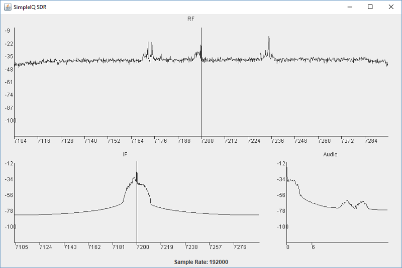
audioFftPanel = new FFTPanel("Audio", sampleRate/4, 0, samples/8, false);I used the ECARS recording to test it. We can see that the IF is now filtered to about +/- 12kHz, which is just inside our Nyquist limit of 24kHz at 48000 samples per second.
If you got this right, the audio sounds good, unchanged in fact. Except now it is playing back at 48000 samples per second and our computer is working less hard.
I took the equation for the Hilbert Transform from Chapter 9 of Lyons' excellent book. He covers the theory and I encourage you to read it, but I will present it here as a magic box, or at least as a Digital Filter that takes in a signal and outputs it with its phase delayed by 90 degrees or PI radians.
Unlike the last digital filter, I am not going to just present the coefficients. Let's implement the filter from the mathematics. That should be our goto approach so that our filters work for different sample rates and bandwidths. We will do that in another tutorial for our other filters.
From Lyons, the equation we will use is this:
sampleRate / (PI * (n-len/2) ) * ( 1 - cos(PI * (n-len/2) ))
Note that I have tweaked his equation. Where he wrote "n", I put n - len/2, where len will be the length of the filter. That will put zero in the center of the response, which is normal for filters. The other way to think about it is that we could run n from -len/2 to len/2 and achieve the same result. His plots of the Hilbert Transform impulse response confirm this is correct.
Also if n == len/2 we are going to have a crash due to a division by zero. The mathematics tells us that we can set the value to zero when n == len/2, so that will need to be in our code.
The code for the Hilbert Transform is almost identical to our FirFilter. We just add a call to init() in the constructor and this builds the filter coefficients. There is no need to store them as a hard coded array.
There are two other things to note. We store the sum of the squares of the coefficient values and then use that as a gain value in our filter. That gives the overall filter a gain of 1. This is very important. Without it our opposite sideband will not be nulled out. Secondly, we have to flip the calculated coefficients before we run the convolution algorithm. That is true for all FIR filters unless their impulse response is symetrical.
So with those notes, here are the constructor and init() method for our HilbertTransform class:
	public HilbertTransform(double sampleRate, int len) {
		init(sampleRate, len);
		M = len-1;
		xv = new double[len];
	}

	private void init(double sampleRate, int len) {
		double []tempCoeffs = new double[len];

		double sumofsquares = 0;

		for (int n=0; n < len; n++) {
			if (n == len/2) {
				tempCoeffs[n] = 0;
			} else {
				tempCoeffs[n] = sampleRate / (Math.PI * (n-len/2) ) * ( 1 - Math.cos(Math.PI * (n-len/2) ));
			}
			sumofsquares += tempCoeffs[n]*tempCoeffs[n];
		}
		gain = Math.sqrt(sumofsquares);///tempCoeffs.length;
		System.out.println("Hilbert Transform GAIN: " + gain);
		// flip
		coeffs = new double[len];
		for (int i=0; i < tempCoeffs.length; i++) {
			coeffs[i] = tempCoeffs[tempCoeffs.length-i-1]/gain;
			//System.out.println(coeffs[i]);
		}

	}
Every time I make a filter I print out the results and graph them. Does it look like the impulse response in the text book? If it does not then go back and try again. So I un-comment the print statements for the coefficients and run the Hilbert Transform constructor from a simple main() method with a statement like this:
HilbertTransform ht = new HilbertTransform(48000, 30);If we cut and paste those 30 values into Excel and chart them we get this, which looks very good. It is the flip of the plot on p488 of Lyons book:
With our Hilbert Transform written we need to address one other issue. When we run our data through any Digital FIR filter, then the data is delayed. This will also happen with the Hilbert Transform. This is in addition to the -90 degree (PI radian) phase shift that we want. To compensate, if we use the Hilbert Transform to phase shift the Q audio, then we run the I audio through the same delay as the FIR filter. It effectively runs through a shift register. We will use a simple class called Delay.java that looks like a filter but just introduces a delay.
Adding our new Hilbert Transform and our Delay are pretty easy. You can see the whole class on github, but all we need to do are add two lines. These go after the decimation and before the audio filter. We then either add or subtract I/Q to get USB or LSB. That seems too easy. Can it possibly work? We might want a bit of gain, but otherwise it should.
		//Demodulate ssb
		audioQ = ht.filter(audioQ);
		audioI = delay.filter(audioI);
		//audio = audioI - audioQ; // USB
		double audio = audioI + audioQ; // LSB
I have got pretty familiar with the ECARS test recording so I play that back through to test this. There are a group of signals from about -20kHz to -30kHz. Start with the Hilbert Transform and Delay commented out. Click at -27234, or if you have the center frequency set to 7200 its at 7173. You can hear a strong signal. But with double sideband we also hear a strong carrier from the upper sideband. Someone is tuning their amplifier. The signal level rises and falls as they adjust the matching of the tubes to the antenna.
Now un-comment the Hilbert Transform and the Delay. Run the same test. The difference is dramatic. The carrier is not just suppressed, it is gone. You can do the same with the signal at -27234. Try clicking to the left of it with and without the side band suppression. Again, its pretty dramatic.
We now have a fairly functional SDR. It's lacking a lot of functions, but it works. The core signal processing chain is solid. We have a clean SSB demodulation. In the next tutorial I will talk about some of the things we need to do for a proper program. Right now we have the audio loop sitting in main. We have tight coupling between the length of the audio loop and our FFTs. We have a somewhat messy relationship between buffer lengths that is easy to get wrong. We will think about our software architecture and address that in the next tutorial.
Prev Tutorial | Index | Next Tutorial
Enter Comments Here:
| On: 05/24/19 13:13 hicham said: |
| Exellent work, nice and clear explanations, keep going, thank you. |
| On: 05/12/20 15:15Nick said: |
Great tutorial, thanks, much appreciated!!
I think I may have spotted a bug in the code
 //Decimate
decimateCount++;
if (decimateCount == 4) {
     decimateCount = 1;
I think decimateCount should be set to 0 otherwise it will take every third sample instead of every fourth.
Do you concur?
|
| On: 05/14/20 16:16 Chris G0KLA said: |
| Well spotted @Nick. That is indeed a bug. Fix it here if you want. It does not
make that much difference but it is important to minimize distortion. In the next
Tutorial you will see how this bug effects the signal and how I fix it.
With that said, I didn't insert this bug on purpose and when I found it and fixed it in the next tutorial I forgot that it was here in the previous one! So many thanks for pointing it out. I should post a warning that the code should not be copied and pasted without reviewing the bug in Tutorial P. |
Copyright 2001-2021 Chris Thompson
Send me an email