
The files for this tutorial are available on github.com/ac2cz/SDR
So far we have created an oscillator, looked at signals on an FFT, played signals back through the sound card and created a simple digital filter. Those are many of the building blocks that we need for our SDR. But there are several blocks we have not yet discussed. We previously showed an SDR block diagram for our SDR, but it simplifies the flow of I/Q samples and how they are mixed to the right frequency.
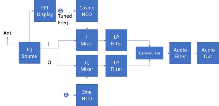
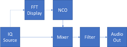
Now we start to delve into how an SDR will actually work, so let's consider the updated flow below. We have an IQ source as before. This now feeds two mixers. We have two oscillators, both set to the same frequency, but one is a cosine oscillator and the other is a sine oscillator. In practice they both look like sine waves, but one is out of phase with the other by 90 degrees. We will call these two Oscillators an IQ Oscillator or a Complex Oscillator. You will also see it called a Quadrature Oscillator. It produces a sine wave with both I and Q components. In this tutorial we will discuss how to build and test the Complex Oscillator. Then we will be ready for Mixing and Demodulation in later tutorials. We will also learn a bit more DSP theory and be better prepared to test our signals and systems in the future.
Lets create a new class, which we will call a complex oscillator, to hold our sine and cosine oscillators. We will also modify our original oscillator so it can produce either a sine wave or a cosine wave.
The complex oscillator is actually pretty easy, despite its name. It stores two oscillators, one called cosOsc and the other called sinOsc. The constructor creates both of them. We have a method to set the frequency, so we can retune after it is created. Our nextSample() method just calls the nextSample() methods on the underlying oscillators. I have then returned the value from nextSample() in a new class called "Complex". We need to return two doubles, one is the cosine (or real part) and the other is the sine (or imaginary part). Together they are a complex number, so we store them in a class called Complex. Also, the only way to return two values in Java is to package them up in a class.
public class ComplexOscillator {

	private CosOscillator cosOsc;
	private SinOscillator sinOsc;

	public ComplexOscillator(int samples, int freq) {
		cosOsc = new CosOscillator(samples, freq);
		sinOsc = new SinOscillator(samples, freq);
	}

	public void setFrequency(double freq) {
		cosOsc.setFrequency(freq);
		sinOsc.setFrequency(freq);
	}

	public Complex nextSample() {
		double i = cosOsc.nextSample();
		double q = sinOsc.nextSample();
		Complex c = new Complex(i, q);
		return c;
	}
}
In the listing above it looks like I have created two new Oscillators classes, but they are both very simple. They inherit almost all of their functionality from the original Oscillator class that we wrote. Here is the whole CosOscillator class, notice the "extends" keyword which means this has all the functionality of Oscillator. When we call "super()" in the Constructor, we call the constructor on the parent class. The SinOscillator class is identical except it builds it calls Math.sin() rather than Math.cos().
public class CosOscillator extends Oscillator {

	public CosOscillator(int samples, int freq) {
		super(samples, freq);
		for (int n=0; n<TABLE_SIZE; n++) {
			sinTable[n] = Math.cos(n*2.0*Math.PI/(double)TABLE_SIZE);
		}
	}
}
To tidy things up we remove the creation of the sinTable from the constructor in Oscillator. We could leave it there, because it gets overwritten by the new classes that inherit from it, but that is wasteful. Having removed that, it is no longer valid to create Oscillator as an object. You need to create either SinOscillator of CosOscillator. So we make the Oscillator class "abstract". Then it can not be created and just serves as a common repository for code that is shared between the two new oscillators we have created.
The start of the Oscillator class, including the constructor, is now:
    public abstract class Oscillator {

	protected final int TABLE_SIZE = 128;
	protected double[] sinTable = new double[TABLE_SIZE];
	private int samplesPerSecond = 0;
	private double frequency = 0;
	private double phase = 0;
	private double phaseIncrement = 0;

	public Oscillator(int samples, int freq) {
		this.samplesPerSecond = samples;
		this.frequency = freq;
		this.phaseIncrement = 2 * Math.PI * frequency / (double)samplesPerSecond;
	}
	...
The only other change I made was to support negative frequencies. This is as simple as allowing the phase to accumulate forward or backwards. That will happen naturally when a negative frequency is passed in. But the nextSample method wraps at 2 Pi, when it is set back to zero. If our frequency is negative we want to wrap at 0 degrees and set it back to 2 Pi. Then I added a new constructor. This means we can call the old constructor and we get an ordinary sine wave oscillator. if we call this new constructor we get to pick either a cosine or a sine wave. So we add two lines to the old method, giving us this:
    public double nextSample() {
		phase = phase + phaseIncrement;
		if (frequency > 0 && phase >= 2 * Math.PI)
			phase = 0;
		if (frequency < 0 && phase <= 0)
			phase = 2*Math.PI;
		int idx = (int)((phase * (double)TABLE_SIZE/(2 * Math.PI))%TABLE_SIZE);
		double value = sinTable[idx];
		return value;
	}
Before we try mixing anything, be better make sure the oscillator works. That is at the heart of our experimental method. Build, test, fiddle, repeat... until it is working.
Let's create a simple main method to test this. Something like the following should do. We will use a simple JFrame to allow us to display two of our LineCharts, one above the other, from the previous tutorials.
public static void main(String[] args) {
int len = 80;
double amp = 1;
int sampleRate = 192000;
double[] bufferI = new double[len];
double[] bufferQ = new double[len];
ComplexOscillator c_osc = new ComplexOscillator(sampleRate, 9600);
JFrame frame = new JFrame();
frame.setDefaultCloseOperation(JFrame.EXIT_ON_CLOSE);
frame.setTitle("Complex Oscillator Test");
frame.setBounds(100,100,700,500);
LineChart plotI = new LineChart("Plot I");
plotI.setPreferredSize(new Dimension(800, 230));
LineChart plotQ = new LineChart("Plot Q");
plotQ.setPreferredSize(new Dimension(800, 230));
frame.add(plotI);
frame.add(plotQ, BorderLayout.SOUTH);
for (int n=0; n< len; n++) {
Complex c = c_osc.nextSample();
bufferI[n] = c.geti() * amp;
System.out.println("I: " + bufferI[n]);
bufferQ[n] = c.getq() * amp;
System.out.println("Q: " + bufferQ[n]);
}
if (bufferI != null) {
plotI.setData(bufferI);
plotQ.setData(bufferQ);
frame.setVisible(true); // causes window to be redrawn
}
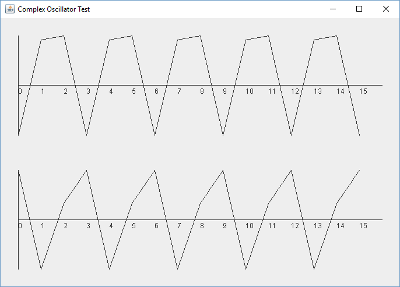
}We run that code and we get something like this:
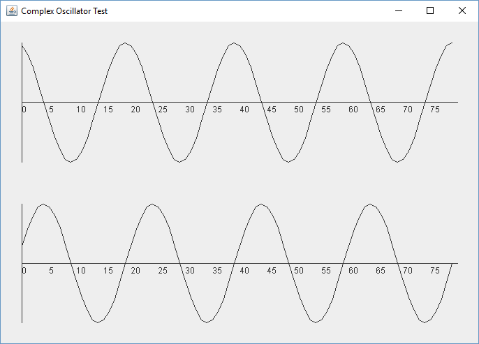
Which looks pretty good. The oscillators start after the first phase increment and we can see that they proceed 90 degrees out of phase. Meaning the sine wave is 90 degrees (or Pi/2 radians) behind the cosine wave. When the cosine wave hits -1, the sine wave is at 0 and falling towards -1. It is 90 degrees behind it. When the cosine has risen back to 0 the sine wave has hit -1, and so it proceeds.
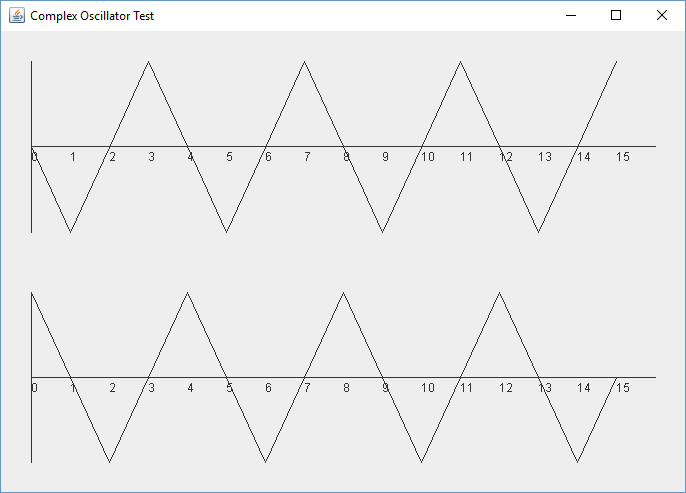
Let's try another frequency. We change the complex oscillator to 48000Hz in our main method and ask it to plot less samples by reducing "len", the length of the data to generate, from 80 to something like 16. After all, there are only 4 samples per cycle for a 48kHz wave sampled at 192kHz. We run it and we get the plot below, which still looks right, though you may find that hard to believe. We appear to have a triangle wave, but it is still 90 degrees out of phase. At 192k samples per second our 48k oscillator has 4 samples per complete cycle. The cosine wave has values 0, -1, 0, 1, 0 and the sine wave has values 0, -1, 0, 1. It is still 90 degrees out of phase.
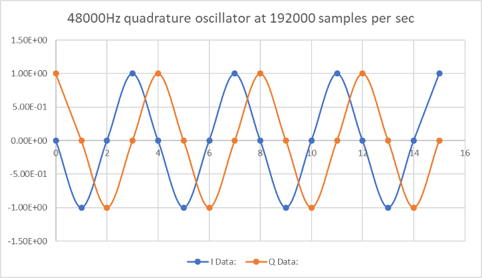
It is also important to realize that it is definitely not a triangle wave. It is still two sine waves. If we take the output into a spreadsheet and plot them, with a curve fitting function, then we get this, which looks exactly right. We know we should fit a curve, rather than assume it is a triangle wave, because a triangle wave (or a square wave) has sharp corners and would not fit in our sample rate. Meaning a 48k triangle wave can not be represented in a 192k sample rate.
Just to be really sure it is all working, let's try a frequency of 90k, which is just inside the Nyquist frequency. The Nyquist frequency is half the sampling rate and the maximum frequency we can sample. By the way, for me, intuitively, it feels like it will not work. It feels like we need at least 4 samples per waveform to represent a phase lag of 90 degrees. The example above at 48kHz feels like it was right on the edge of what is possible. That is not the case of course, as we shall see.
Changing the sample rate to 90kHz, we get the following plot. It's hard to tell if it is working so we plot it in Excel again. This time it fails to fit a sine wave, given the sparse number of samples. Perhaps that is expected. But inspection of the first 4 samples of each wave and even an attempt to draw the curve by hand shows that it does indeed seem to be broken. This is not two sine waves 90 degrees apart. What happened? Is our intuition correct? Do our oscillator only work for lower frequencies? A sine wave just below the Nyquist limit only has two samples per cycle. Can we really represent two different sine waves 90 degrees apart with such sparse data points? It does not seem like it could possibly work.
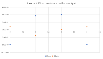
My adventure into DSP has been full of this sort of mind twister. If you are an old hand, you know the answer. Of course it will work. Two sample points can represent any sine wave below the Nyquist frequency. So we can precisely define two sine waves 90 degrees out of phase.
If you had skipped this testing step and implemented this in your code as the local oscillator, then it works, but not quite. And not in all situations. And it has some noise. It does not balance out the sidebands. It's one of those DSP bugs where it works just well enough for you to not know what is broken. This emphasizes the importance of testing each component to make sure it works as expected. Finding this error in an end to end SDR would be much harder.
It turns out that the bug is relatively easy to fix. When we accumulate our phase we check if we have wrapped around the end of the sine wave. If we have, then we start back at 0 phase and proceed through the lookup table. That does not work as the frequency increases. For a sine wave that has only two samples, the first phase of each sample is not zero degrees. It is already part way into the sine wave and changing each time we loop around two PI radians.
So we need to update the code to add or subtract 2 Pi radians each time we wrap around the sine cycle, instead of resetting. The updated method is like this:
public double nextSample() {
phase = phase + phaseIncrement;
if (frequency > 0 && phase >= 2 * Math.PI)
phase = phase - 2*Math.PI;
if (frequency < 0 && phase <= 0)
phase = phase + 2*Math.PI;
int idx = (int)((phase * (double)TABLE_SIZE/(2 * Math.PI))%TABLE_SIZE);
double value = sinTable[idx];
return value;
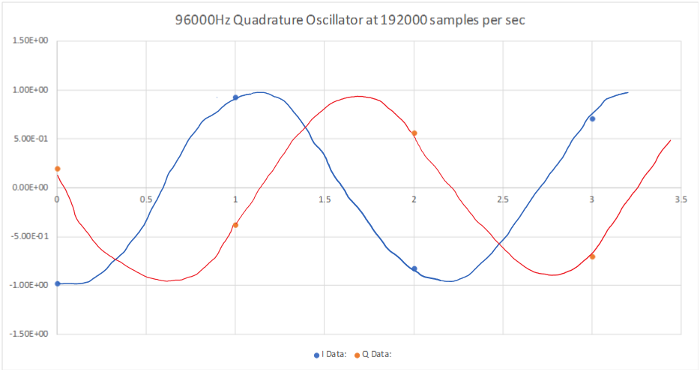
}When we run this and plot it, at first it looks worse. We have a triangle wave that changes in amplitude. But we ignore that, knowing that our LineChart can not fit the right curve. So we extract the samples into Excel and plot them. I drew the curve in by hand because Excel again can not fit a curve. We see they look much better. Even though there are only two samples per cycle we can draw the cosine and sine waves in and it looks very good. This will work as our oscillator.
I didn't fake this bug to make a point. It came out of my own testing. Subtle bugs like this are all over DSP code. It's impossible to write a good program without testing each piece. With our complex oscillator now working, we will use it in the next tutorial to mix our signals down to base band.
But our testing is not over. We need to look at the frequency response of oscillator to make sure it is good. That will take us into a bit more DSP theory as we try to understand if it is working.
We have also touched here on the minimum number of samples needed to represent a sine wave in our DSP code, but it is worth noting that our intuition is not wrong. Two samples for a sine wave is ambiguous. It can represent an infinite number of waves. All of the duplicates are above the Nyquist frequency. For that reason the Nyquist frequency is also called the folding frequency because our frequency spectrum starts to repeat due to aliases of our samples. There are an infinite number of repetitions of our data as we go up in frequency. This will become important when we convert from one sampling rate to another in the future.
With what looks like good amplitude response, let's review the oscillator in the frequency domain. We will use almost the same main method, but we change our LineChart to our FFTPanel from the last tutorial. We sample 1024 values to give us a decent frequency resolution.
public static void main(String[] args) {
int len = 1024;
double amp = 0.01;
int sampleRate = 192000;
double[] buffer = new double[2*len];
ComplexOscillator c_osc = new ComplexOscillator(sampleRate, -6000);// 4800 6000
JFrame frame = new JFrame();
frame.setDefaultCloseOperation(JFrame.EXIT_ON_CLOSE);
frame.setTitle("Complex Oscillator Test");
frame.setBounds(100,100,1000,500);
FFTPanel plot = new FFTPanel(sampleRate, 0, len, true);
frame.add(plot);
for (int n=0; n< len; n++) {
Complex c = c_osc.nextSample();
buffer[2*n] = c.geti() * amp;
buffer[2*n+1] = c.getq() * amp;
}
if (buffer != null) {
plot.setData(buffer);
frame.setVisible(true); // causes window to be redrawn
}
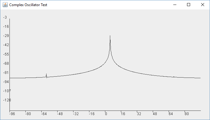
}I put -6000Hz as the first frequency to test and it looks like this, which could not be more perfect. It is in the negative frequency range and it is a nice narrow impulse at the right frequency!
Feeling good I put in 5000Hz and uh-oh, that looks bad!
What is going on here?
First of all it is not +ve/-ve frequencies. 6kHz and -5kHz would show the same results. The first thing to realize is that 192000 / 6000 = 32, Meaning it is an exact division of the sample rate and a power of 2 division at that. 192000 / 5000 = 38.4.
What has happened is that the 5kHz oscillator is sitting between two sample bins and its frequency spectrum is bleeding or smearing into other sample bins. The 6kHz oscillator is not because it sits exactly on a bin. But a quick check of 4800Hz, which does divide exactly, also shows this issue. So it is not as simple as sitting on a bin. So what is going on here? And is this a fatal flaw? Does our DSP code need to somehow stick to a finite series of bins?
First of all, this is a display issue of the FFT. It is not necessarily a problem with our underlying oscillator, which can represent any frequency we want below the Nyquist frequency. But this issue is preventing us from being able to analyze it, so we need to understand and address it.
Our problem stems from the unavoidable fact that the DFT operates on infinite series of data. Or at least the mathematics does. Our computer does not. The -6kHz wave happens to look exactly the same at its start and end. It enters and leaves the 1024 samples we are feeding into our FFT (at 192000 samples per second) as though it is a continuous wave. The amplitude and phase are the same at the start of the 1024 samples as they are at the end. So it may as well be an infinitely long continuous wave. This is what the DFT requires if you remember the theory.
Our 5kHz wave does not fit in the same way. The start of the 1024 samples and the end have a different amplitude and phase. The FFT mathematics assume that the 1024 samples we have taken repeats immediately after this chunk in exactly the same way. When we take the FFT we are looking at a static chunk of data that is supposed to represent the infinitely long wave. If you think about the end of the 1024 samples wrapping around and starting again with the beginning of the 1024 samples, then there is a discontinuity. The wave jumps. That jump is a frequency and phase response. The FFT has to calculate it and plot it out. We see the result of that discontinuity in the results.
These issues are annoying because our data is not really like this. So how do we proceed?
The answer is we fake an infinite series of data. In the DSP literature you will see statements such as "apply a window to the data".
Our chunk of data, the 1024 samples, is a window of the data in DSP parlance. We are looking at just a section of it through a window. When we truncate our data, as we have done here by simply extracting 1024 samples, we call it a square window. That means the data starts and stops abruptly. The FFT of a square window is a broad peak with an infinite series of diminishing peaks to either side. It looks like the below:
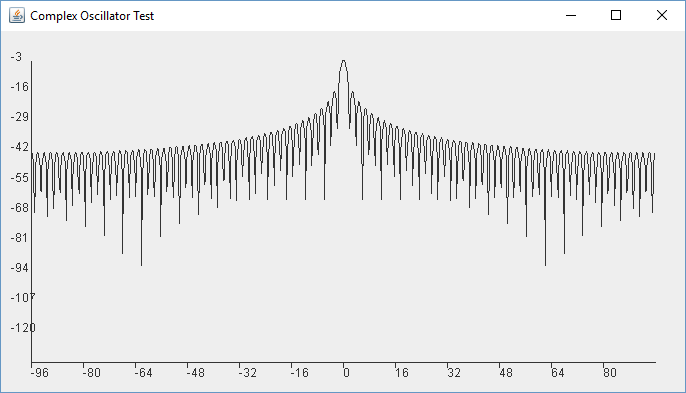
By the way, you can recreate that square window by putting a series of 1s in the middle of the data you process through the FFT, while leaving the other values as 0 and then run the FFT. It makes this cool plot. Who would have thought that such a simple data structure could create something that looks so beautiful.
But our square window, beautiful or not, has been multiplied by our data. That may not seem obvious, but it is a fact. Mathematically, if we end up with a worst case amplitude jump as we wrap around from the end of our data chunk and back to the start, then it looks like we multiplied all of our data elements by 1 and everything outside our data sample is multiplied by zero. The FFT assumes the data is infinite and it looks like we have a narrow sample set in the middle of an infinite number of zeros. Furthermore, DSP theory includes this important relationship:
Multiplication in the time domain is the same as convolution in the frequency domain
Convolution in the time domain is the same as multiplication in the frequency domain
So when we (accidentally) multiplied our data by a square window, it means we convolved our frequency response with the frequency response of the square window. That convolutions is the same convolution calculation we used in the previous tutorial on filtering, except now our Frequency Domain values are being updated. When our input data fitted exactly into 1024 samples with no discontinuity, the impact of the convolution was hidden. For all other values we see it. The effect is almost literally on/off. Try putting in 6001. Just 1 Hz off.
The solution is to use a "window" that gently ramps up and ramps down our data. Then it starts and ends at the same amplitude and phase. DSP theorists have invented many windows for this purpose but we will only use a couple. For now let's use a Blackman Window. We can find the (slightly scary looking) formula from a DSP textbook. We could implement it in a method in our Tools class, but let's put it in a Window class because we may have other Windows and methods to implement in the future. For now it just has one method. I put it in the Signal package.
public class Window {

	public static double[] initBlackmanWindow(int len) {
		double[] blackmanWindow = new double[len+1];
		for (int i=0; i <= len; i ++) {
			blackmanWindow[i] =  (0.42 - 0.5 * Math.cos(2 * Math.PI * i / len)
					+ 0.08 * Math.cos((4 * Math.PI * i) / len));
			if (blackmanWindow[i] < 0)
				blackmanWindow[i] = 0;
		}
		return blackmanWindow;
	}
}
We update our main method to create the window and to apply it to our data, by adding the follow lines
    double[] bmw = Window.initBlackmanWindow(len);
    ...

    buffer[2*n] = buffer[2*n] * bmw[n];
    buffer[2*n+1] = buffer[2*n+1] * bmw[n];
    ...
If we run that for 5000Hz again it looks better. The peak is narrower for what looks like 40dB or even 50dB. That is a good range but the plot is far from perfect. There are some other strange peaks. If we tweak our FFTPlot class to extend the range and plot all of the data, it becomes unclear if this is actually better. If we put in other frequencies sometimes there are many peaks. Is that an issue? Is our oscillator broken? This does not look like the plot from a spectrum analyzer...
Counter-intuitively, these plots are hard to read because they have no noise in them. If we were looking at the results of a real oscillator with a spectrum analyzer we would not be able to see results at -200dB or more. We do our best to remove all the noise from our analog equipment, but there is a noise floor regardless. Here we have no noise and the plot looks very strange.
In our actual SDR there will be plenty of noise from the antenna. To analyse our oscillator more realistically and to make it easier to examine the data, we add some noise. I will call it "dither", which, as well as "indecisive", the dictionary defines as "add white noise to (a digital recording) to reduce distortion of low-amplitude signals". A simple Java method will return us a random number that we can add to our data. We put it in main and it looks like this:
private static double dither() {
    return Math.random()/1000000;
}We call our dither() method from main by updating our window multiplies like this:
buffer[2*n] = buffer[2*n] * bmw[n] + dither();
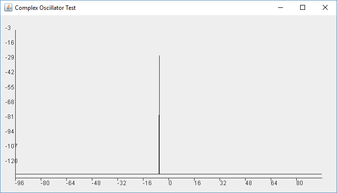
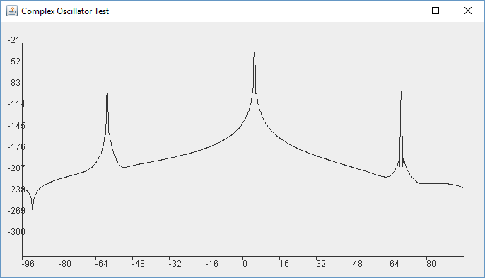
buffer[2*n+1] = buffer[2*n+1] * bmw[n] + dither();If we run our main method again for 5000Hz we get the below, which finally looks more like we would expect.

Note that adding the noise (dither) has given us a spike at 0Hz. This is 1/f noise and is virtually unavoidable. It has risen out of the random data that we added. A bit spooky and another strange feature of information theory. Note that in an SDR we can largely remove the DC spike by averaging the FFT.
Also, we can still see the spikes either side of our data. So these are a real issue or artifact from our oscillator. You will see them called spurs. They are at -70dB, with our peak at -30dB. So they are 40dB down. In a homebrew analog oscillator we might be happy with that, but we can do better. These spurs are a result of phase inaccuracies in our oscillator. When we calculate the phase increment we then lookup the nearest value in our lookup table. If the value is not exact then we get spurs like this from the small frequency jumps. The jumps are small shifts and look like additional high frequencies in our data stream. The frequencies are outside our Nyquist frequency, but they alias here in our spectrum. In a homebrew radio we might filter the oscillator and we could do that here. But we will consider a different approach.
If we change our lookup table to have 9600 values (vs 128 or even vs 1024) then the spurs disappear into the noise at -120dB. So we do that. The only cost is the space for the lookup table. That might be important on an embedded computer, but it is not an issue for a modern desktop or laptop. You can also try other frequencies to see if there are any other spurs.
That is about it for the ComplexOscillator class. In the next tutorial we will use it to mix our signal down to baseband.
Prev Tutorial | Index | Next Tutorial
Enter Comments Here:
| On: 10/07/25 15:15 said: |
Copyright 2001-2021 Chris Thompson
Send me an email