
The files for this tutorial are available on github.com/ac2cz/SDR
If you have ever built a direct conversion receiver then you know that once you mix the signal from the antenna with the local oscillator then you are left with audio. You just need to filter and amplify that audio, then you can pipe it out of a speaker or some headphones. As I said in Tutorial 3 it's not a great receiver. It is double sideband and all of the selectivity has to be with audio filters, which need large inductors and are not very selective. But it is simple and fun to build.
At the start of sdr_tutorial3 we went back to Tutorial 2 and fed the output of the Funcube Dongle or whatever SDR you are using into the FFT and we could see the spectrum. What would happen if we had just fed that output through the sound card and listened to it? Well there is only one way to find out. (Note this next part will only work if your sound card can play 192k samples per second audio. Most can. If it cannot, then you will need to decimate the audio first to 48k samples per second. More on that in a future tutorial.)
Let's create a new class that takes audio and plays it out of the speaker. Luckily this is very simple if we use the default sound card. In fact our new AudioSink class will be almost exactly the same as the SoundCard class, except TargetDataLine is replaced by SourceDataLine. A SourceDataLine is Java's terminology for an output device we can write to. I guess the device itself is sourcing its data from us. I don't know who came up with the back to front naming convention.
We have the same, but opposite, piece of complexity that we found in SoundCard. Our internal representation for audio is a double from -1 to 1. We need to write to the sound card as bytes in the format required by the sound card. So we create a utility routine to do that and store it in the Tools class. We will want to be able to seamlessly go back and forward between these formats. The conversion is not complex, but it does need to deal with both mono and stereo streams and needs to unpick a double into two bytes. You can see the new routine in the updated Tools class.
Here is the new AudioSink class:
package tutorial4.audio;

import javax.sound.sampled.AudioFormat;
import javax.sound.sampled.AudioSystem;
import javax.sound.sampled.DataLine;
import javax.sound.sampled.LineUnavailableException;
import javax.sound.sampled.SourceDataLine;
import tutorial4.signal.Tools;

public class AudioSink {

	AudioFormat audioFormat;
	SourceDataLine sourceDataLine;
	boolean stereo = true;

	public AudioSink(int sampleRate) throws LineUnavailableException {
		audioFormat = SoundCard.getAudioFormat(sampleRate);
		DataLine.Info dataLineInfo = new DataLine.Info(SourceDataLine.class, audioFormat);
		sourceDataLine = (SourceDataLine) AudioSystem.getLine(dataLineInfo);
		sourceDataLine.open(audioFormat);
		sourceDataLine.start();
	}

	public void write(double[] f) {
		byte[] audioData = new byte[f.length*audioFormat.getFrameSize()];
		boolean stereo = false;
		if (audioFormat.getChannels() == 2) stereo = true;
		// assume we copy MONO stream of data to stereo channels
		Tools.getBytesFromDoubles(f, f.length, stereo, audioData);
		write(audioData);
	}

	public void write(byte[] myData) {
		sourceDataLine.write(myData, 0, myData.length);
	}

	public void stop() {
		sourceDataLine.drain();
		sourceDataLine.close();
	}
}
With the audio sink coded, we can update our main class for Tutorial 3, make a copy of it and modify it just slightly. We set sampleRate to 192000 and len, the number of samples to grab from the audio source, to 4096. We add the AudioSink and each time we read from the sound card we write that data to the audio sink. We are using the SoundCard and WavFile classes that were updated in Tutorial 3 so they take "stereo" as a paramater so that we can process the Complex FFT in FFTPanel.
We can't write the stereo data that we source to the output sound card. It is not really stereo audio. It is two channels of audio, with one delayed by 90 degrees. For now we will ignore that and just take one of the channels. Now we have a mono channel of real audio. We can write that out directly through the AudioSink. Note that if we want to look at the FFT of our audio data instead of the FFT of our complex IQ data then one channel of our FFT needs to be set to zero. Try toggling that line on/off after you have run the code to see what difference it makes. Effectively we are using the Complex FFT to give us a real only result. The documentation for JTransforms confirms this is valid. For the RealForward method is says "you will get the same result as from complexForward called with all imaginary parts equal 0".
public static void main(String[] args) throws UnsupportedAudioFileException,
	IOException, LineUnavailableException {
		int sampleRate = 192000;
		int len = 4096;
		//WavFile soundCard = new WavFile("ecars_net_7255_HDSDR_20180225_174354Z_7255kHz_RF.wav", len, true);
		SoundCard soundCard = new SoundCard(sampleRate, len, true);
		MainWindow window = new MainWindow("SimpleIQ SDR", sampleRate, len);

		AudioSink sink = new AudioSink(sampleRate);
		FirFilter lowPass = new FirFilter();

		double[] audio = new double[len];
		boolean readingData = true;

		while (readingData) {
			double[] buffer = soundCard.read();
			if (buffer != null) {
				for (int d=0; d < audio.length; d++) {
					audio[d] = buffer[2*d];
					buffer[2*d+1] = 0;
				}
				sink.write(audio);
				window.setData(buffer);
				window.setVisible(true); // causes window to be redrawn
			} else
				readingData = false;
		}
	}
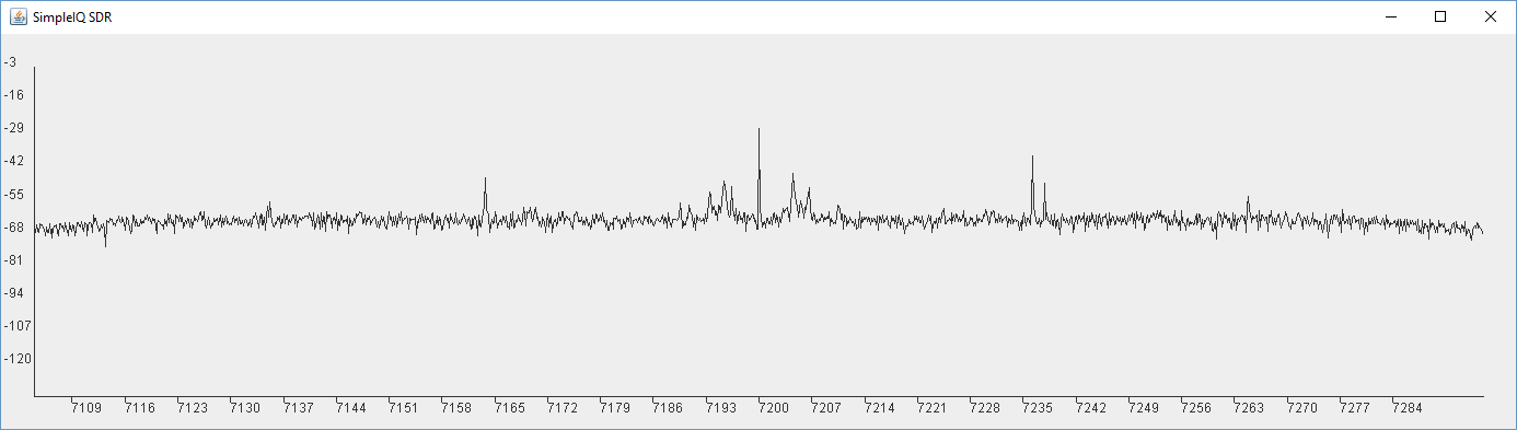
To test it I used another program to set the center frequency of my FCD SDR to 7200kHz and then ran the program. I used the other program to retune the center frequency as needed. Again, you can setup the default sound card for audio input and output in your OS. In Windows you go to "Manage Audio Devices" from settings or the Control Panel and on the Playback tab make sure that the default recording and playback devices are the ones you want. If one of them is not, select it and click "Set Default". In a future tutorial we will add this selection process to our program.
With that done I ran it and wow! I can hear signals. The FFT result no longer looks the same if we compare to HDSDR or another SDR program. We see that is is symmetrical and it has all of the signals above and below the center frequency on both sides. In fact we can ignore one side and just look at the right hand side. There is no additional information to the left. This is because we are looking at real audio and not a complex IQ signal.
What is more, we can now hear ALL of the signals at the same time, at least those that fit into the hearing range of my ears. Given this is SSB, we hear signals above the center frequency as upper sideband and those below as lower sideband. Effectively we have the positive and negative frequencies overlaid. The audio of the negative frequencies sound as though we have selected the wrong sideband on our radio. This means half of the signals are unintelligible squarks. The other half are at various frequencies from Donald Duck to audible by dogs only. But some we can hear and the parts we hear are very clear. It really reminds me of a basic homebrew direct conversion receivers, with bright audio, no AGC and a large range of signal strengths.
In fact, as we listen and look closer, we notice that the stations we hear are shown in the FFT display very close to the center, which makes sense. If nothing is audible, try retuning until a signal is just to left of the center on the 3rd party SDR. We are hearing signals that are in the audio range from 0 - 20kHz. If we compare to an HDSDR output or a similar SDR, we also see that the signals we can actually hear are all to the left of the center frequency, so the negative frequencies. This makes sense too because the signals on 40m phone are Lower Sideband.
So that was fun. It shows us that the data we are getting from one channel of the the IQ radio is really audio, just a very wide bandwidth, and that it has positive and negative frequencies mixed in. Remember, we are examining this as ordinary audio by looking at just one channel, so we can't tell the negative frequencies from the positive ones.
Before we look at both I and Q, in an effort to separate positive frequencies from negatives (USB from LSB), what happens if we follow the design of the hardware direct conversion receiver and add some filtering?
Let's add a very basic digital filter. This is not how our SDR will work eventually, but it is a good experiment and will help us understand how filters work.
A cursory inspection of the DSP literature shows us that there are two main types of digital filters Finite Impulse Response (FIR) and Infinite Impulse Response (IIR). For now we will implement an FIR filter because they are easier to understand and code. Later we will see that IIR filters are better in some situations and FIR in others.
An FIR filter uses a set of coefficients stored in an array in Java. Those coefficients are called the filter kernel or sometimes the filter taps. The filter is implemented by sliding the set of coefficients along the audio samples and performing a calculation called convolution. This requires us to multiply each coefficient by the corresponding audio sample and then add the results together.
As an example, let's look at a data stream with two sine waves jumbled together in it. I generated 20 samples of a 1200Hz tone and 10kHz tone using the Oscillator from Tutorial 1. I simply added the results together from the two oscillators, with the 1200Hz tone scaled to amplitude 0.5 and the 10kHz tone scaled to 0.1 amplitude. That gives us a list of values like this:
0.17,0.20,0.14,0.19,0.35,0.50,0.49,0.40,0.40,0.50,0.59,0.53,0.38,0.33,0.35,0.39,0.29,0.10,0.01,0.00
If we plot those 20 values we get the first half cycle of the 1200Hz wave, because it is 40 samples long at 48000 samples per second (48000 / 1200 = 40):
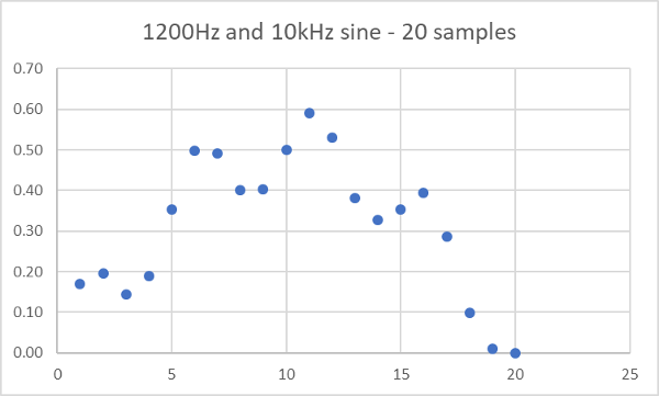
It looks pretty noisy. More like a mountain range than a sine wave.
As our filter kernel we use the following 5 values, which are designed to filter at 0.06 of the sampling rate (this is the cut off frequency), or in this case 48000 * 0.06 = 1.44 kHz.
0.12,0.13,0.13,0.13,0.12
One thing to remember about DSP is that everything is relative. This filter will sample at 0.06 of the sample rate regardless of what that is. So it will work just the same for 192000 samples per second, giving a cut of rate of 192000 * 0.06 = 11.5kHz.
To calculate the first filtered value we imagine our data as shown below. Note that we pad the start with 4 zeros. We perform all the multiplies shown vertically and then add each together horizontally to give the result 0.02:
0.12,0.13,0.13,0.13,0.12
  *    *    *    *    *
0.00,0.00,0.00,0.00,0.17,0.20,0.14,0.19,0.35,0.50,0.49,0.40,0.40,0.50,0.59,0.53,0.38,0.33,0.35,0.39,0.29,0.10,0.01,0.00
                      =
                    0.02
We carry on in this way. For the next calculation we slide the filter kernal to the right as shown below and results in 0.04:
     0.12,0.13,0.13,0.13,0.12
       *    *    *    *    *
0.00,0.00,0.00,0.00,0.17,0.20,0.14,0.19,0.35,0.50,0.49,0.40,0.40,0.50,0.59,0.53,0.38,0.33,0.35,0.39,0.29,0.10,0.01,0.00
                           =
                    0.02,0.04
If we do that for all of the values then plot the results, we get this:
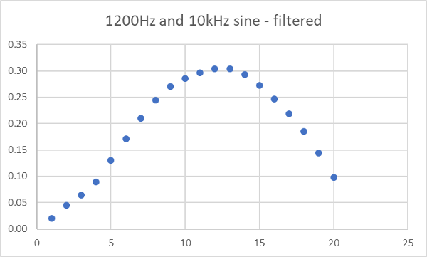
Which to me is almost like magic. We have mostly recovered the 1200Hz sine wave by multiplying our stream by 5 numbers. We have filtered out the 10kHz tone.
Ok, so magic aside, where did the 5 numbers come from? There are several answers to that.
From an engineering perspective we can use a Filter Calculator to create the coefficients from parameters like the cut off frequency, the filter prototype and the number of coefficients you require. I like the Iowa Hills Filter Design Software but that is sadly only available in the internet archive now. There are many other options. I used a raised cosine prototype, a filter cutoff of 0.06 and asked for 5 coefficients.
As we get deeper into our SDR we will find that filters need to be variable width. They need to work with different sampling rates. They need to be updated at run time. For that we will need to understand more of the theory, including the mathematical calculations needed to rebuild the filter kernel. But that can wait for now.
The other answer I could have given is that the kernel is the impulse response of the filter, meaning it is the shape of the waveform that is created when the input is a single impulse. I could have also said that the kernel is the inverse Fourier Transform of the desired Frequency Domain response. Digital Filters are fascinating and I encourage you to read more about them.
Fascinating or not, Digital Filters are only useful if they work. Let's add one to our test and see what happens. In fact we can just use this simple test filter because 192000 * 0.06 = 11.5kHz. So the cutoff frequency of this test filter will do nicely to start with.
First we need a simple filter class that implements the convolution and stores the kernel values. Let's create an FirFilter class like this. Note that I have given the full values calculated for the filter coefficients.
package tutorial4.signal;

public class FirFilter {

	double coeffs[] = {
			0.117119343653851,
			0.129091809713508,
			0.133251953115574,
			0.129091809713508,
			0.117119343653851
	};

	double[] xv;  // This array holds the delayed values
	double gain = 1;
	int M; // The number of taps, the length of the filter

	public FirFilter() {
		M = coeffs.length-1;
		xv = new double[coeffs.length];
	}

	public double filter(double in) {
		double sum;
		int i;
		for (i = 0; i < M; i++)
			xv[i] = xv[i+1];
		xv[M] = in * gain;
		sum = 0.0;
		for (i = 0; i <= M; i++)
			sum += (coeffs[i] * xv[i]);
		return sum;
	}
}
The class has one complexity, the filter method. This takes one double and returns it after the convolution with the filter kernel. We store a delayed copy of our data in the array xv so that the calculation works each time we call the method.
We update our main method with just a couple of extra lines. We add a "lowPass" filter object, which is the instantiation of our FirFilter class. We then call the filter() method on lowPass each time we read an audio buffer. The results are written to the speaker and displayed with the FFT. So we add lines like this:
	FirFilter lowPass = new FirFilter();

	...

	for (int d=0; d < audio.length; d++) {
		//audio[d] = buffer[2*d];
		audio[d] = lowPass.filter(buffer[2*d]);
		buffer[2*d] = audio[d];
		buffer[2*d+1] = 0;
	}
	...
Let run that with and without the filter (by changing which line is commented out) to see and hear the difference. I get the two plots below. The first is with the filter the second is without:
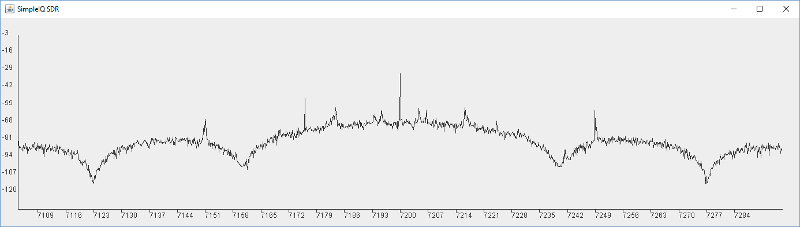
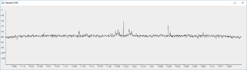
If you tried this and listened to the audio you will hear a real difference between the two, which is amazing for so simple a filter. But it's far from perfect. We see the filter has a very gentle roll off with a couple of deep nulls. We can still hear a lot of the interference and high frequencies. We can see that clearly in the Frequency display from the FFT. While there are some good deep nulls, most of the response is not that suppressed. Also note the crazy lumpy response. This is characteristic of a raised cosine digital filter.
If we go back to our filter designer and update the length of the filter to 32 or 64 we will see a much better response. If we update our filter coefficients to the following, then it is immediately better:
double coeffs[] = {
			-0.006907390651426909,
			-0.005312580651013577,
			-0.002644739091749330,
			 0.001183336967173867,
			 0.006192514984703184,
			 0.012327624024018900,
			 0.019453074574047193,
			 0.027354594681004485,
			 0.035747363433714395,
			 0.044290256550950494,
			 0.052605352818230700,
			 0.060301340430963822,
			 0.066999061029964030,
			 0.072357178973056519,
			 0.076095892581739766,
			 0.078016723675218447,
			 0.078016723675218447,
			 0.076095892581739766,
			 0.072357178973056519,
			 0.066999061029964030,
			 0.060301340430963822,
			 0.052605352818230700,
			 0.044290256550950494,
			 0.035747363433714395,
			 0.027354594681004485,
			 0.019453074574047193,
			 0.012327624024018900,
			 0.006192514984703184,
			 0.001183336967173867,
			-0.002644739091749330,
			-0.005312580651013577,
			-0.006907390651426909
	};
This is the result of a slightly longer 32 coefficient filter:
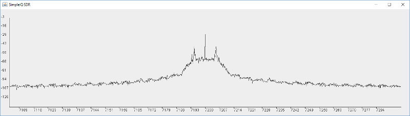
If we play with the filter calculation software, we see that we can get 60dB of suppression if the filter is 128 coefficients long, but the roll off is slow and we only get that by about 12kHz. Those coefficients are also in the FirFilter class file if you want to play with them. It is far from a perfect filter, but when we run it we get a nice sounding audio.
That introduces filtering, which will become very important to us. We will see new filters in a later tutorial, including filters that can be changed at run time as we updated the bandwidth required. In the next tutorial we will discuss the architecture needed for our SDR and the updated Oscillator we will need to feed the mixers.
Prev Tutorial | Index | Next Tutorial
Enter Comments Here:
| On: 04/08/20 13:13 Claude KE6DXJ said: |
| I believe I have successfully worked through Tutorial 3 but in starting Tutorial 4 I think I need some further help distinguishing between the two sources of I&Q data. Based on cost, I chose to use the RTL-SDR V3 dongle rather than the Fun Cube Dongle. As a result, I think I am receiving raw (rf) I&Q 8 bit bytes. I think my question concerns the idea of turning this raw I&Q data into a format that can generate audio as the beginning of Tutorial 4 suggests. Does Fun Cube Dongle produce I&Q audio data or am I missing some basic understanding of this I&Q data? So far I have not involved the sound card portion of these tutorials because of this confusion on my part. Any thoughts would be appreciated. Thanks, Claude PS: Should I move this discussion to a direct email rather than through the tutorial? |
| On: 04/08/20 14:14 Claude KE6DXJ said: |
| I should have included some additional information. I am using the rtl_sdr.exe command line tool to capture (into a file) the I&Q data directly from the RTL-SDR V3 dongle rather than a third party software package like SDRSharp.exe. This could be part of my confusion. |
| On: 04/08/20 15:15 Chris G0KLA said: |
| Hi Claude, glad you finished Tutorial 3. The key to using rtl_sdr.exe will be to understand the format it produces. From this page https://osmocom.org/projects/rtl-sdr/wiki I think it produces alternating bytes for I and Q. In tutorial 2 I showed a routine to convert the bytes into doubles. This situation is simpler because it is only 1 bytes, or 8 bits. They have a value from 0-256. You will need to treat 127 as zero and scale the bytes to a value from -1 to 1. So perhaps subtract 127 and divide by 256. Once you have the data converted into doubles you should be able to treat it like audio data. Pick a narrow bandwidth to start with, like 240,000 samples per second. So you are not overloaded with too much data. |
Copyright 2001-2021 Chris Thompson
Send me an email