
The files for this tutorial are available on github.com/ac2cz/SDR
Before we dive into the world of Quadrature Signals, we need to decide what hardware we will use for our software defined radio. We have several approaches we can take.
For this tutorial we are going to assume that I and Q audio is available on the stereo channels either read from a sound card or from a wav file. That means you have either built your own radio, are sourcing audio from a sound card based SDR like the Funcube Dongle or are using IQ audio from a third party SDR. If you have a different USB dongle then for now I suggest you open that in another SDR program and record some audio into an IQ file. You can then open the IQ file and process the data in these tutorials. We will frequently record audio and process from a wav file rather than directly from hardware because it is more repeatable and easier to debug. But note one thing. If your SDR is very wide bandwidth and you record that full bandwidth, then you may have difficulty with some of the earlier tutorials. Later we will show how to reduce wide bandwidths to a manageable size with decimation. For now record at a bandwidth like 192000 samples per second.
You can also use my test file if you are unable to record your own.
Let's try to create the most simple IQ radio we can, using just the tools we have so far.
Our architecture will be as follows:
In the above architecture we have an IQ Source which supplies I and Q on the stereo channels of the sound card. Or we are reading I and Q samples from a wav file. We read the data into an FFT and display it. We can see the frequency that we will decode on the display and this frequency is passed to the Numerically Controlled Oscillator (NCO). The NCO feeds a software mixer which combines the output of the NCO with the IQ source. We then filter and output the results to the speaker or other sound card device.
People with experience homebrewing radios will recognize this as a direct conversion receiver. If you replace the IQ source with a Low Noise Amplifier (LNA), if the FFT display is replaced with a knob and dial and the NCO is replaced with a VFO, then we have a classic receiver. In fact if you have never built one of these with an NE602 and an LM386, then you should go do that. It is amazing what you can achieve with a handful of components.
A direct conversion receiver with a handful of components is a marvel, but it is not a high performer. It is double sideband, so we have every signal twice at slightly different frequencies. We get interference from stations that are on the other side of zero beat. The filtering is not sharp because it has to be done at audio frequencies. All of those problems are solvable in hardware, but with complex solutions. I built a very nice direct conversion transceiver for example, but you end up with a high component count.
Fortunately those issues are solvable in software with less complexity and with much higher performance. I won't say they are easily solved, or that it is trivial, because there are plenty of things that can go wrong. Some things, like filtering out the opposite side band are much easier in software, but other things, like understanding the Complex FFT results, require some work.
Perhaps you already did this. What happens if we just set our IQ source as the default sound card and run it in Tutorial 2? Or if we have a recording of IQ data, what happens if we let it run through Tutorial 2?
We need to make a couple of tweaks first. We set the "sampleRate" value in the main method to 192000 and increase "len", the size of the samples and FFT length, to 4096.
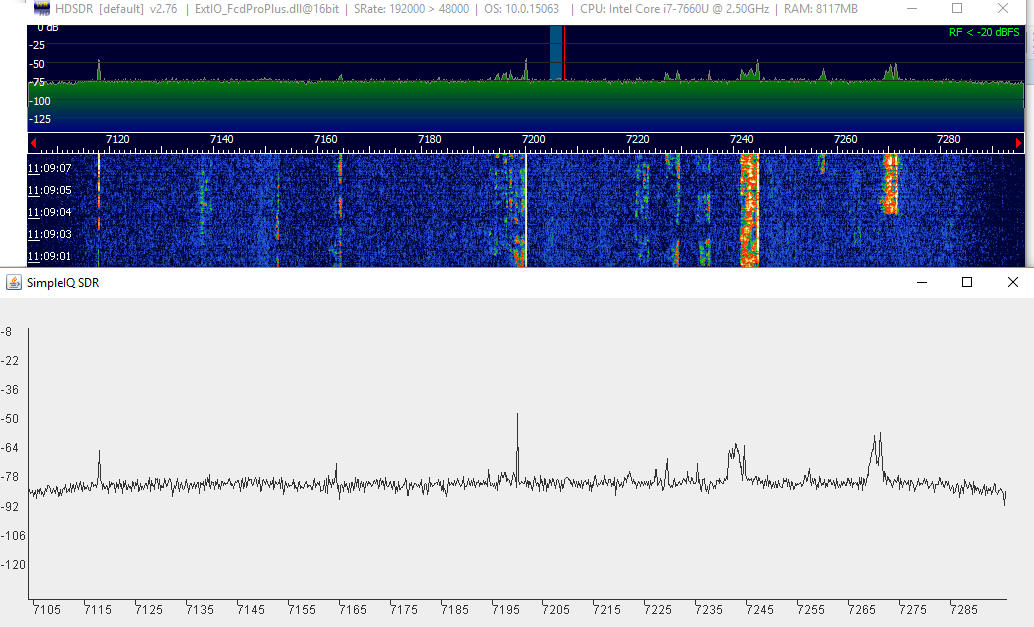
I am using a Funcube Dongle. I used another SDR to set the local oscillator frequency to 14020kHz, right in the middle of the CW section of the 20m band. I like HDSDR because it produces very good recordings, but you can use another 3rd party SDR if you like.
With that all setup, I ran the program again and get the following displayed in our LineChart:
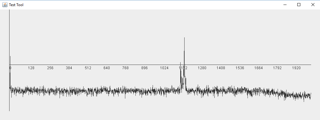
That looks pretty interesting, but is it right? Does it show us anything meaningful? Let's compare that to what we see in something like HDSDR:
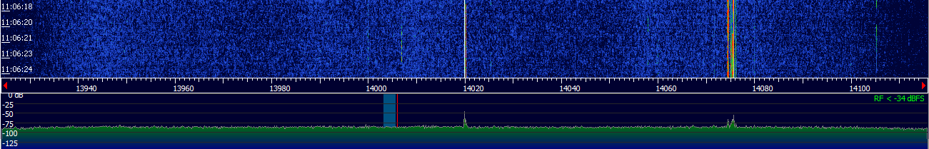
Hmm, it is not immediately obvious that they are the same, but it turns out they are. Sort of. Click on the images to make them bigger if you need to inspect them. It looks like our LineChart is just showing the right hand part of the display. On the HDSDR FFT we have a central DC spike at 14020. The local oscillator is the center frequency of our display. To the right of the DC spike we have a set of signals at about 14075kHz. This is the current craze for the digital mode FT8, so 14075 sounds about right. Our real FFT in our LineChart shows the local oscillator frequency in bin 0 on the left hand side of the display. It then shows the same FT8 signals starting about bin 1152. We calculate the bin bandwidth as 192000/4096 = 46.875Hz. So bin 1152 is an offset of 54000Hz or 54kHz. 14020 + 54 is 14074kHz. So these are definitely the same signals.
All this math is a bit tedious. We will update our display tool to show frequency shortly, but we first need to understand why we only have half of the spectrum that HDSDR has.
Our test took one stereo channel from the sound card and calculated the real FFT of it. HDSDR is taking both stereo channels, I and Q, and then calculating the Complex FFT. The result is twice as much bandwidth centered on the local oscillator. But that is not all. Look what happens if I change the local oscillator and have some clear signals on either side of the center frequency:
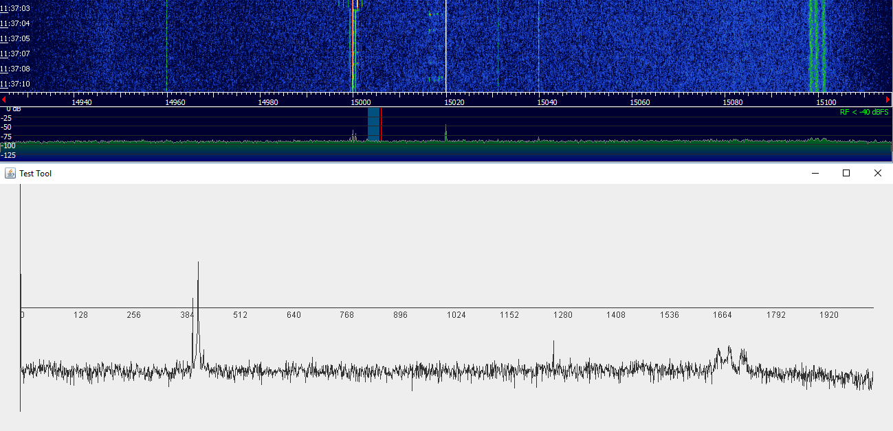
Uh, oh. We see the signals that HDSDR has on either side of the center frequency in our LineChart display. Except they are all on one side. It turns out that running the real FFT on one stereo channel has recreated the simple hardware direct conversion receiver in software. It is double sideband and the sidebands are 96kHz wide.
The solution to this is actually the same if we are building a high performance direct conversion receiver with electronic components or if we are building it in software. The incoming signal has already been split it into I and Q, which just means we have our signal and a copy of our signal delayed by 90 degrees or PI radians. The delayed signal is called the Quadrature Signal and is referred to as Q. We then process both I and Q to recover our signals. In that way we can demodulate any type of signal we want.
Let's create a class to display a chunk of IQ data as a nice FFT result. This will be based on LineChart. We could extend it, but it is a such a simple class that we will make a copy and modify it from there. Our new class will be called FFTPanel.
Before we get deep into FFTPanel, we need to understand the Complex FFT, at least somewhat. As you read this it may all sound a bit, well, complicated. You don't need to understand everything but you do need to know how the data is laid out and how to calculate the magnitude and phase results. If we remember back to the Prev Tutorial the FFT algorithm was used to implement the real DFT, which decomposed our N signal samples into N/2+1 Cosine waves and N/2+1 Sine waves. We referred to the cosine and sine waves as the Real and Imaginary components of the signal.
In the Complex DFT both our input and output will have cosine and sine wave components.
For the input, the I input is the amplitude of the Cosine wave and is the real component while Q is the amplitude of the Sine wave and the imaginary component. Remember I said that Q is delayed 90 degrees, well a sine wave is 90 degrees out of phase with a cosine wave.
When we run the Complex FFT our output or frequency domain result again has real and imaginary parts. In the real DFT we just looked at the first half of the result. The other half is not calculated by the JTransforms real DFT because it is the mirror image. In the complex DFT the second half contains the negative frequencies.
Now negative frequencies sound a bit strange but as Radio Amateurs we are quite familiar with them. If we take an oscillator and mix it with an incoming signal we expect to get both Upper and Lower sideband signals, unless we filter one of them out. In that case we have both positive and negative frequencies in the mixing operation. We have exactly the same situation here. The Local Oscillator in our SDR has been mixed with the signal from our antenna. Our bandwidth is 192kHz, so we have 96kHz of positive and 96kHz of negative frequencies on either side of the local oscillator frequency. We can not display that with the real DFT because you can not distinguish positive frequencies from negative ones, but we can with the complex DFT.
In our program we will need to double the size of the input and output array, as shown in the layout below. For example, with a 16 point Complex FFT the input array needs to store 32 values. The output is also 32 values and then the Power Spectral Density (PSD) will be length 16.
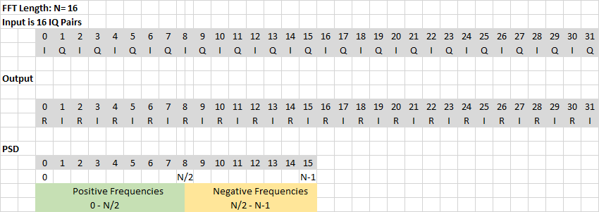
The positive frequencies are stored in PSD bins 0 to N/2 and the negative frequencies are stored from N/2 to N-1. This is not the same layout that we will display to the user. We would expect the negative frequencies to be on the left, not the right. Bin 0 is our local oscillator frequency. Bin N/2 is half the sample rate.
It is worth knowing that our spectrum is periodic, meaning that our bins from N/2 to N-1 hold the same values as the bins from -N/2 to 0 (if we had calculatled them). So we can see that the negative frequencies do sit to the left of the local oscillator signal, but mathematically they repeat and the FFT algorithm stores the negative frequency results in the bins from N/2 to N-1. It is also worth knowing that all sampled spectrum are periodic. That is part of the weird world of DSP. It is also something we will need to take into account and we will discuss more when that is the case.
So, that is all we need to know for now. There is more in the DSP guide and other books, which I encourage you to read. Let's move on to the code to implement this.
So armed with this information, we copy LineChart and modify it. Let's change the constructor and the setData method to setup and do the FFT calculation. This is "refactored", which is a fancy term for moved, from our previous main method. The good news is that it also got simpler. We had a special calculation in the DFT for the Power Spectral Density values at the start and end. It turns out that is not needed in the complex FFT where we can treat all results the same. Like before, we again average the results.
	public FFTPanel(int rate, long freq, int length) {
		sampleRate = rate;
		centerFrequency = freq;
		fftLength = length;
		binBandwidth = sampleRate/fftLength;
		psdBuffer = new double[fftLength+1];
		fft = new DoubleFFT_1D(fftLength);
	}

	public void setData(double[] buffer) {
		fft.complexForward(buffer);
		for (int k=0; k<buffer.length/2; k++) {
			double psd = Tools.psd(buffer[2*k],buffer[2*k+1], binBandwidth);
			if (firstRun)
				psdBuffer[k] = psd; // we do not have an average yet
			else
				psdBuffer[k] = Tools.average(psdBuffer[k], psd, averageNum);
		}
		firstRun = false;
		this.data = psdBuffer;
		repaint();
	}
We also rewrite the paint routine. Much of the changes are pedestrian display code which have nothing to do with DSP, and you can see the rest of the changes in the FFTPanel class. The core is the display of the FFT itself, which is shown below. Notice that we draw it in two halves with the negative frequencies first. We have some tricky offsets to make sure that we scale bin numbers to the right location on the screen. We use the same "getRatioPosition()" routine that we wrote for LineChart. In fact we made it "static" which means we can reference it without instantiating a LineChart object.
	// Draw the FFT result, one half at a time
		// First the negative frequencies, which we will draw on the left
		for (int n=fftLength/2; n< (fftLength); n+=step) {
			int y = LineChart.getRatioPosition(minValue, maxValue, data[n], graphHeight);
			int x = LineChart.getRatioPosition(fftLength/2, 0, n-fftLength/2, graphWidth/2);
			x = x + BORDER;
			gr.drawLine(lastx, lasty, x, y);
			lastx = x;
			lasty = y;
		}
		// Then the positive frequencies, which we draw on the right
		for (int i=0; i< (fftLength/2); i+=step) {
			int y = LineChart.getRatioPosition(minValue, maxValue, data[i], graphHeight);
			int x = LineChart.getRatioPosition(fftLength/2, 0, i, graphWidth/2);
			x = x + BORDER + graphWidth/2;
			gr.drawLine(lastx, lasty, x, y);
			lastx = x;
			lasty = y;
		}
In addition to the display loop, we change the axis labels. First we don't want to automatically scale the Y axis. For this test we pick a range of values from 0 to -120 and then plot the FFT result against that. One immediate question is why the Y axis magnitude values are negative. The answer is, because they are very small and we are showing the log value. We use log because they have a large range and are difficult to plot and visualize as raw values. The values we are plotting are the magnitude of the bin (sqrt ( Re^2 + Im^2) divided by the bin bandwidth. So we are showing the power for one Hz. The values are all less than 1. The log of a value less than 1 is negative. You can think about this as power in dBm/Hz.
Secondly, we want the X axis to be labeled with frequencies based on the center frequency of the SDR. To keep everything neat, I put the routines that draw the axis in two private methods "drawHorizontalScale" and "drawVerticalScale". The only real complexity is calculating the frequencies given the positive and negative values. In the routine that draws the scale, we simply calculate the lower and upper bounds from the center frequency and then plot the labels from smallest to largest.
	private void drawHorizontalScale(Graphics gr, int graphWidth, int zeroPoint) {
		int minFreqValue = (int) (getCenterFreqkHz()-sampleRate/2000);// half the bandwidth in kHz
		int maxFreqValue = (int) (getCenterFreqkHz()+sampleRate/2000);// half the bandwidth in kHz
		int labelWidth = 50; // allow 50 pixels per label
		int numLabels = (graphWidth) / labelWidth;
		int increment = (maxFreqValue - minFreqValue) / numLabels;
		int label = getCenterFreqkHz()-increment*numLabels/2; //freq value for this label
		gr.drawLine(BORDER, getHeight()-BORDER, BORDER, BORDER); // axis line
		for (int v=0; v < numLabels; v++) {
			int pos = LineChart.getRatioPosition(maxFreqValue, minFreqValue, label, graphWidth);
			gr.drawString(""+label, pos+BORDER, zeroPoint+15);
			gr.drawLine(pos+BORDER, zeroPoint, pos+BORDER, zeroPoint+5);
			label = label + increment;
		}
	}
The "drawVerticalScale" method is similar. You can see both of them in the FFTPanel class. With those created it is time to test it. I decided to modify the MainWindow class so that it passes the sampleRate, centerFrequency and FFT length into the FFTPanel class. That may be how we do it in the future, so it seems like a good way to go.
import javax.swing.JFrame;
import tutorial3.plot.FFTPanel;

@SuppressWarnings("serial")
public class MainWindow extends JFrame {

	FFTPanel fftPanel;

	public MainWindow(String title, int sampleRate, int samples) {
		super(title);
		this.setDefaultCloseOperation(EXIT_ON_CLOSE);
		setBounds(100, 100, 1400, 400);
		fftPanel = new FFTPanel(sampleRate, 7200000, samples);
		add(fftPanel);
	}

	public void setData(double[] data) {
		fftPanel.setData(data);
	}
}
As a result, our main method becomes very simple. In fact this sort of approach where we code, test, and then refactor to make the code more readable and maintainable, is very common.
	public static void main(String[] args) throws UnsupportedAudioFileException,
	IOException, LineUnavailableException {
		int sampleRate = 192000;
		int len = 4096;
		//WavFile soundCard = new WavFile("ecars_net_7255_HDSDR_20180225_174354Z_7255kHz_RF.wav", len, true);
		SoundCard soundCard = new SoundCard(sampleRate, len, true);
		MainWindow window = new MainWindow("SimpleIQ SDR", sampleRate, len);

		boolean readingData = true;
		while (readingData) {
			double[] buffer = soundCard.read();
			if (buffer != null) {
				window.setData(buffer);
				window.setVisible(true); // causes window to be redrawn
			} else
				readingData = false;
		}
	}
You may have noticed that SoundCard and WavFile now take an extra parameter, a boolean. Our current implementation extracts one stereo channel and returns it as doubles. We now want both stereo channels. Rather than just modify the code to provide both channels, we pass in a paramater so we can either extract one channel or both.
We need to modify the constructor, because this changes the size of the array that is returned, and the read method. SoundCard and WavFile get modified in the same way, here are the updated methods for SoundCard:
	public SoundCard(int sampleRate, int samples, boolean stereo) throws LineUnavailableException {
		readBuffer = new byte[samples * 4];
		if (stereo)
			out = new double[samples * 2];
		else
			out = new double[samples];


		audioFormat = getAudioFormat(sampleRate);
		DataLine.Info dataLineInfo = new DataLine.Info(TargetDataLine.class, audioFormat);
		targetDataLine = (TargetDataLine) AudioSystem.getLine(dataLineInfo);
		targetDataLine.open(audioFormat);
		targetDataLine.start();
		this.stereo = stereo;
	}

	public double[] read() {
		targetDataLine.read(readBuffer, 0, readBuffer.length);
		for (int i = 0; i < out.length; i++) {
			int step = 4;
			if (stereo) step = 2;
			byte[] ab = {readBuffer[step*i],readBuffer[step*i+1]};
			double value =  Tools.littleEndian2(ab,16)/32768.0;
			out[i] = value;
		}
		return out;
	}
Let's run our new program. I set the center frequency in HDSDR to 7200kHz, the center of the phone portion of the 40m amateur band in the US. I then set the center frequency to 7200000 in the MainWindow call to FFTPanel and executed the program. We should get something like the below, shown side by side with the output from HDSDR:
Prev Tutorial | Index | Next Tutorial
Enter Comments Here:
| On: 07/24/19 17:17 Alfred leon said: |
| Hello! When do you talk about "Tutorial x" (USB Dongle)? Thanks for all! |
| On: 07/24/19 18:18 Chris g0kla said: |
| Hi Alfred, thanks for the comment. Unfortunately I have not written Tutorial X yet. If you want to be notified when it is written then send me an email (address at bottom of page). I'll then email you when it is ready. |
| On: 05/11/20 15:15 Claude KE6DXJ said: |
| After working on Tutorial 4 for some time, I started to suspect that my
implementation of some of the Tutorial 3 modules contained some problems.
While working through these questions, I compiled your Tutorial 3 code from
Github. One bit of code, that both my code and (I think) your code, had the
same issue. It has to do with computing the average Power Spectral Density
(PSD) values from the Power Spectral Density (PSD) values. Collecting the
output values from the initial and the average computation showed no change.
There is a one for one identify between the two outputs.
After running some test cases on simple data arrays, I suspect that the Tutorial 3 FTPanel method that calculates the PSD and also calls Tools.average has the issue. I think the method setData in FTPanels calls the Tools.average method with the same value for the first parameter (average value) and the second value (new sample) resulting in no change to the average value. Should it call the Tools.average with the previous average (psdBuffer[k-1]) and current value with the new sample computed from the fft buffer (Buffer[k*2]) or the PSD buffer previously computed (psdBuffer[k]). This is a snip of the FTPanel.setData code with the change:
firstRun = false;
for (int k=0; k<buffer.length/2; k++) {
     double psd = Tools.psd(buffer[2 * k], buffer[2 * k + 1], inBandwidth);
     if (firstRun) {
          psdBuffer[k] = psd; // we do not have an average yet
     } else {
          psdBuffer[k] = Tools.average(psdBuffer[k-1], psd, averageNum);
}
Not sure this is clearly expressed. I can provide data collection text files with the before and after outputs. I have accounted for the initial pass PSD computation and the final average PSD computation. As an aside, I stole a moving average sample code from the internet with a different implementation and its output matched the modified FTPanel.setData output. This code used a nested loop to compute the new average for each new sample. |
| On: 05/11/20 17:17 Claude KE6DXJ said: |
| Maybe the special characters in the code snipet are preventing it's printing. Let me know if (and how) to provide more information if it is required. |
| On: 05/11/20 18:18 Chris G0KLA said: |
| Hi @Claude, yes the < character was preventing the rest of the code snippet
from printing, because its part of the HTML tags. I was surprised that happened
because my web page comments typically run through a script that cleans that
sort of thing up, but I guess this page does not have that for some reason. I
will investigate.
But on to your question... I don't think the average algorithm is wrong. It does not use the "previous average value" by taking the previous value in the array. The array holds a snapshot of the entire spectrum. So the value at psdBuffer[k] is the average power value for "bin" k of the FFT. When we calculate a new average using the fast average algorithm we pass in the previous average for that bin. So it is right to pass in psdBuffer[k] to calculate a new value of psdBuffer[k]. Let me know what issue you see with you code and I'll try to help. This stuff is not easy, so there are no stupid questions! |
Copyright 2001-2021 Chris Thompson
Send me an email