
The Java files for this tutorial are available on github.com/ac2cz/SDR
The Python files are on github.com/ac2cz/pySdr
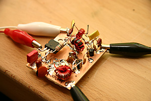
Perhaps the first homebrew project I built that was not directly from a kit was an oscillator. They are a key part of the radio architecture, perhaps as a VFO or as a crystal oscillator for a mixer. This is a good place for us to start our adventure into software defined radio.
Like homebrew electronics, we need to be able to measure and see the results of our experiments. On the test bench we have a DVM, an oscilloscope and perhaps a spectrum analyzer. We also use a radio (software defined or otherwise) to hear and see our signals.
Let's create an oscillator and a piece of test equipment that we can use to measure it.
An analog oscillator typically has a tuned circuit and we pick C and L values to set the frequency. In the digital realm we do not produce a continuous wave, but instead deal with samples. Each sample is represented by a number. We will use values between -1 and 1 to represent our signals. You will see other formats and we will have to convert to/from them for storage in files or to pass in and out of hardware sound cards. But more on that later.
We need to be able to see the results of what we do. One approach is to print out values and graph them. This will get us started. Given everything is digital we can cut/paste and graph with a spreadsheet. Later we will add some code to draw graphs on the screen and eventually use that as part of our radio.
So we start with a simple oscillator. Let's say we want a sine wave at 1200Hz.
In software our sine wave generator is called a Numerically Controlled Oscillator or NCO. In Java or Python we can create this with a short class called Oscillator which has one constructor that takes the requested frequency, the sample rate in samples per second and then builds a table of sine values. This will save us from calculating the sine value every time we need a sample of our waveform.
The frequency is relative to the sample rate and is used to set the amount that the phase increases for each sample. One complete sample of our waveform has 2 pi radians. We define the phase increment as 2 pi times frequency / samples per second. That means our 1200Hz wave will make one complete cycle in 48000 / 1200 = 40 samples
Finally, we create a method called nextSample (note that in Python I will follow the typical naming convention using lower case and underscores for functions/methods, so it will be next_sample). We will call nextSample each time we need a new sample of our waveform.
Pulled together in a class it looks like the below.
If you want to work in Python, click the bar below to show the example Python code, otherwise click Java.
If you are new to Python then have a look at my Quick Python Tutorial. In Python the Oscillator class goes in a file called Signal.py. That makes it a Python module, which we can include in another Python program with the import keyword.
import math

class Oscillator:
    TABLE_SIZE = 128

    def __init__(self, frequency, samples):
        self.freq = frequency
        self.sampleRate = samples
        self._phase = 0
        self._sinTable = self._init_table()
        self._phaseIncrement = self._calc_phase_inc(self.freq, self.sampleRate)

    def _init_table(self):
        table = []
        for n in range(0, self.TABLE_SIZE):
            table.append(math.sin(n*2.0*math.pi/self.TABLE_SIZE))
        return table

    def _calc_phase_inc(self, frequency, samplesPerSecond):
        return 2 * math.pi * frequency / samplesPerSecond

    def next_sample(self):
        self._phase = self._phase + self._phaseIncrement
        if (self._phase >= 2 * math.pi):
            self._phase = 0;
        idx = (int)((self._phase * self.TABLE_SIZE/(2 * math.pi))%self.TABLE_SIZE)
        value = self._sinTable[idx]
return valueIf you are new to Java have a look at my Quick Java Tutorial, which will explain that each class goes in its own source file. We must therefore name the file Oscillator.java, to match the class name. I have given it the package name "signal" and therefore stored it in a sub-directory called signal. I have also put all of the files in a package "tutorial1". You don't have to use packages if you don't want, but as our collection of classes grows, it is helpful for them to be organized into packages. That said, you probablly don't want to put everything in a top level package called tutorial1. Change that to something like sdr or whatever you called your project. I used the tutorial pacakges so I can show the progress of the classes as we moved from tutorial to tutorial. You don't need to do that.
package tutorial1.signal;

public class Oscillator {

	private final int TABLE_SIZE = 128;
	private double[] sinTable = new double[TABLE_SIZE];
	private int samplesPerSecond = 48000;
	private int frequency = 0;
	private double phase = 0;
	private double phaseIncrement = 0;

	public Oscillator(int samples, int freq) {
		this.samplesPerSecond = samples;
		this.frequency = freq;
		phaseIncrement = 2 * Math.PI * frequency / samplesPerSecond;
		for (int n=0; n<TABLE_SIZE; n++) {
			sinTable[n] = Math.sin(n*2.0*Math.PI/TABLE_SIZE);
		}
	}

	public double nextSample() {
		phase = phase + phaseIncrement;
		if (phase >= 2 * Math.PI)
			phase = 0;
		int idx = (int)((phase * TABLE_SIZE/(2 * Math.PI))%TABLE_SIZE);
		double value = sinTable[idx];
		return value;
	}
}
Note: there is a bug in this code which we discover and fix in Tutorial 5. It is fine for this tutorial, but don't cut/paste this code for other purposes without reading about the bug.
Having created the oscillator, let's write a very short program to call it.
In our test we will simply create an instance of the Oscillator with the sample rate set to 48000 and the frequency set to 1200. We will then call it in a loop to output the values that are generated. We can then graph the values in a spreadsheet to see if they look right.
Python does not have to have a main() method. It will just execute any code that is not inside a class or function. That said, by convention the entry point for the Python program is often called main() and I will follow that.
import signal

def main():
    buffer = []
    sample_len = 100
    osc = signal.Oscillator(1200, 48000)
    for n in range(0, sample_len):
        buffer.append(osc.next_sample())
        print(buffer[n])

main()A program in Java has to have a class with a method called main() in it. This is the entry point for the program. The class it goes in can be called anything. (In fact we can add a main() method as a quick entry point to any class for testing). Note that if the file Oscillator.java is in the same directory and package as your main class, then you will not need the import statement for Oscillator
package tutorial1;
import tutorial1.signal.Oscillator;

public class SdrTutorial1 {

	public static void main(String[] args) {

		Oscillator osc = new Oscillator(48000, 1200);

		int len = 100;
		for (int n=0; n< len; n++) {
			double value = osc.nextSample();
			System.out.println(value);
		}
	}
}
When we run the program it prints out 100 values of the waveform. I pasted them into excel and while the values were still highlighted I clicked Insert > Scatter Plot Chart, which plotted the values. The commands may be different in another spreadsheet, but you should be able to plot them.
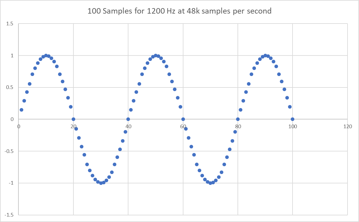
What we get looks great! We see two complete cycles of the waveform in the first 80 samples. But is that what we expect?
At 48000 samples per second, a 1200Hz tone would take 48000 / 1200 = 40 samples for a single cycle. So this looks good! It represents a 1200Hz tone at 48000 samples per second. This is the experimental method applied to SDR. We have created our oscillator, run it in a test situation and measured the results. The results agree with our theory. This is often not the case of course. Typically when I create some new code it does not do what I expect. So this experiment and measure approach is critical to make sure it is working.
One final note. If we arbitrarily decide this set of numbers are samples at 96000 samples per second, then this is a 2400Hz tone because it completes one cycle in 40 samples. 96000/40 = 2400. There is no change to the numbers or the file. Everything in DSP is relative to the sample rate. This can be confusing if you are new. There is nothing in the numbers that "stores" the sample rate in some way.
Let's finish by running some analysis on the signal using one more test tool. We will often want to look at the frequencies in our signal both to understand if our radio is working and to display the results to the user. On the electronics test bench we would use a spectrum analyzer. In software we use a Fourier Transform.
There are lots of explanations of the Fourier Transform. I like the detailed explanation in The Engineers and Scientists Guide to DSP. In fact the whole book is recommended and is available online for free.
We will use the Fast Fourier Transform (FFT) which is an algorithm that efficiently implements the Discrete Fourier Transform or DFT. Don't worry too much about the names. The DFT is just the Digital equivalent of the Fourier Transform. The FFT is not another different transform, it is just a way to implement it.
The Fourier Transform decomposes the signal into a set of component sine and cosine waves. Specifically the numbers that it returns are the magnitudes of those sine and cosine waves. The sine and cosine waves span the frequencies from 0 to half our sampling rate. The magnitude of each sine and cosine represents the magnitude of our signal at those frequencies. In fact the sines and cosines collectively are our signal. We can literally add them back together and get our signal again.
This decomposition allows us to analyze the signal as its component frequencies and to visualize them. We get to see the spectrum. We have all seen this either on a spectrum analyzer, on a pan adapter or on the waterfall of an SDR.
Before we jump in, we need to understand the output that we will get. We will supply 128 samples and the real FFT will return 65 results. The results are in pairs made up of Real (Re) and Imaginary (Im) values. The real parts are the amplitudes of the cosine waves that make up our signal and the imaginary parts are the amplitudes of the sine waves. They are called Real and Imaginary to match the algorithm for the Complex DFT, which returns Complex numbers, even though the results from the Real DFT are real numbers. For the real DFT this is just a convenient way of returning the results, but it is confusing. Don't worry about it for now, just think of it as a way to pack and return the data from the algorithm.
We don't typically look at the Cosine (Real) and Sine (Imaginary) magnitudes when we are doing frequency analysis. We are instead interested in how we can use them to calculate the actual Magnitude of our signal at each frequency and the corresponding Phase. We can calculate those from the Cosine (Real) and Sine (Imaginary) magnitudes as follows:
	mag[k] = sqrt( Re[k]^2 + Im[k]^2)
	phase[k] = arctan (Im[k]/Re[k])
If that is also confusing, then don't worry. You have to understand the results of this and not necessarily all of the mechanics. If you want to understand more, then it is well explained in Chapter 8 of the Engineers and Scientists guide to DSP.
Continuing our experimental method we expand our main routine so that we can calculate and print the magnitude of the FFT. We store the calculated NCO values in a buffer and then run our FFT with the values in the buffer. We change the length to 128 because the FFT works best with lengths that are a power of 2. You can also see that we calculate the magnitude of each frequency using two results, rather than display the actual returned values.
In Python we will use the FFT implemented in the numpy module. Specifically we will use the real FFT. This takes a list of doubles as input and returns a list of complex numbers. In this case they are not really complex numbers. The real part of each complex number contains the magnitude of the cosine wave and the imaginary part contains the magnitude of the sine wave.
If you do not already have numpy installed, then do that now. If you are new to all this then see my Python Tutorial
I have also used matplotlib to show the FFT plot. It is a useful tool for quick plots like this, though we will shortly write our own widget because we want to be able to interact with it. You can also print the values and create the plot in a spreadsheet again, saving you the installation of matplotlib
import matplotlib.pyplot as plt
import signal
import numpy as np
import math

def main():
    buffer = []
    sample_len = 128
    osc = signal.Oscillator(1200, 48000)
    for n in range(0, sample_len):
        buffer.append(osc.next_sample())
        print(buffer[n])
    #plt.plot(buffer, label='1200Hz')
    out = np.fft.rfft(buffer)
    psd = []
    psd.append(out[0].real)
    half = int(len(out))
    for k in range(1, half):
        psd.append(math.sqrt(out[k].real*out[k].real + out[k].imag*out[k].imag))
    psd[half-1] = math.sqrt(out[0].imag*out[0].imag + out[half-1].imag*out[half-1].imag)
    plt.plot(psd, label='FFT')
    plt.show()
main()In Java we will use the excellent JTransforms FFT library. Specifically we will use the realForward method which calculates the real DFT of our data. Note that the DoubleFFT_1D API has the following to say about the method and the result set:
	public void realForward(double[] a)
	Computes 1D forward DFT of real data leaving the result in a. The physical layout of the output data is
	as follows:

	if n is even then:

	 a[2*k] = Re[k], 0<=k<n/2
	 a[2*k+1] = Im[k], 0<k<n/2
	 a[1] = Re[n/2]

	This method computes only half of the elements of the real transform. The other half satisfies the
	symmetry condition. If you want the full real forward transform, use realForwardFull. To get back the
	original data, use realInverse on the output of this method.
Note there is a slightly special treatment for the "bins" at 0 and n/2.
If you are trying to build this and have an issue including the JTransforms library, then see my Java Tutorial for instructions on including external jar files.
package tutorial1;
import org.jtransforms.fft.DoubleFFT_1D;
import tutorial1.signal.Oscillator;

public class SdrTutorial1 {

	public static void main(String[] args) {

		Oscillator osc = new Oscillator(48000, 1200);

		int len = 128;
		double[] buffer = new double[len];
		for (int n=0; n< len; n++) {
			double value = osc.nextSample();
			buffer[n] = value;
		}

		DoubleFFT_1D fft;
		fft = new DoubleFFT_1D(len);
		fft.realForward(buffer);
		System.out.println(buffer[0]); // bin 0
		for (int k=1; k<len/2; k++)
			System.out.println(Math.sqrt(buffer[2*k]*buffer[2*k] + buffer[2*k+1]*buffer[2*k+1]));
		System.out.println(Math.sqrt(buffer[1]*buffer[1] + buffer[len/2]*buffer[len/2])); // bin n/2

	}
}
I ran the program, then cut/pasted the calculated values into a spreadsheet and plotted them as a scatter plot. It is shown below:
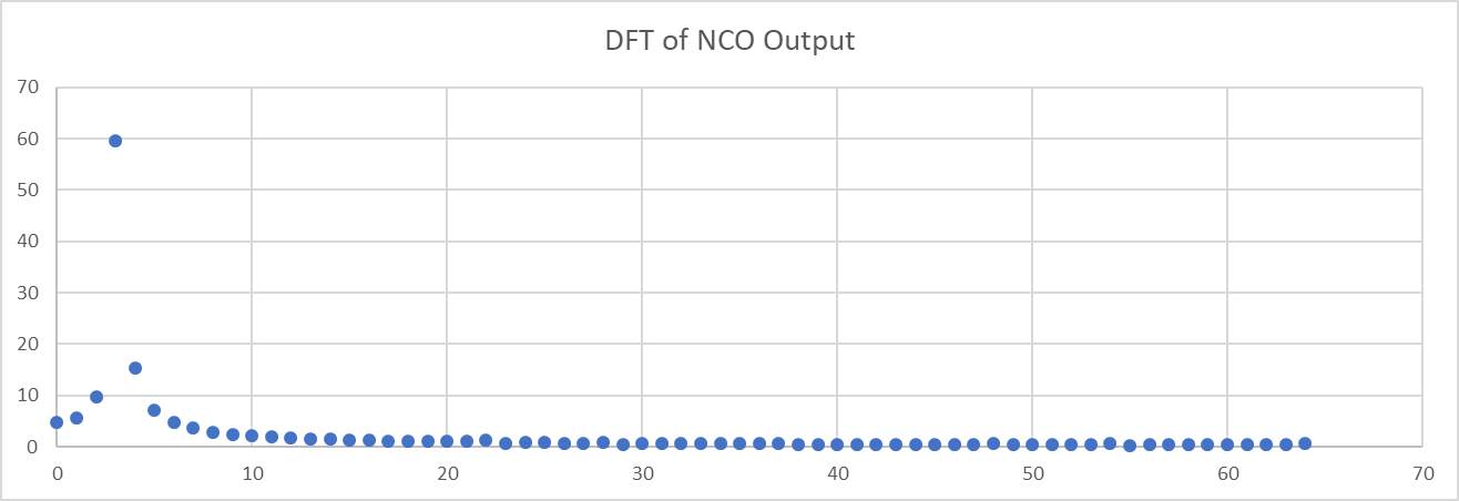
Wow! That is pretty exciting. We have a set of 65 result values, which we call "bins", from 0 to 64. We ran an FFT with 128 points, which returned 65 cosine (real) and 65 sine (imaginary) values. We have calculated the magnitude for each bin from the combination of the cosine (real) and sine (imaginary) values. We then see that bin 3 (counting from bin 0) is dramatically raised.
What do the bins mean? Bin 0 holds the DC component of the signal. Bin 1 represents a cosine and a sine wave that each make one cycle in the FFT length. So bin 1 represents a cosine and sine wave that are 128 samples long at 48000 samples per second, so they have 48000/128 = 375 cycles in a second, which is 375Hz. That means bin 3 represents the magnitude of our signal at 3 * 375 = 1125Hz and bin 4 shows the magnitude at 1500Hz. That seems pretty convincing for our 1200Hz tone. We have plotted the spectrum of our oscillator!
With that said, why are many other bins raised up? This might surprise us, given we generated a very pure single frequency in software. Shouldn't it be infinitely thin? Instead we see numerous bins around our target frequency raised. We won't be able to understand why without beginning our tumble down the rabbit hole of DSP.
Note: Don't use this oscillator, because it has a bug, which we will discover and fix in Tutorial 5. No need to post about it in the comments below :)
Enter Comments Here:
| On: 01/28/19 0:00 matrixmike said: |
| I am enjoying working through the tutorial, though, yay, I have just started |
| On: 01/28/19 10:10 Chris / g0kla said: |
| Great to hear @matrixmike. Let me know if you have questions. |
| On: 05/09/19 11:11 Daniel KK4MRN said: |
| Wow! What a great tutorial on SDR and DSP. I am following along but writing my stuff in C#. Maybe later I will redo it in Go lang as well. |
| On: 05/09/19 13:13 Chris g0kla said: |
| Glad it is helpful Daniel. Let me know if you see any mistakes or things that are hard to follow - relatively speaking of course - because all of this is a bit hard to follow :) |
| On: 05/18/19 16:16 Mistake in Java code for the test of the oscillator for tutorial 1 said: |
| The frequency and samplesPerSecond are backwards in the test code in Java. This results in an array of all zeros. However, the test code in Python works correctly. Patch for the Java test: Before: Oscillator osc = new Oscillator(48000, 1200); After: Oscillator osc = new Oscillator(1200, 48000); |
| On: 05/18/19 17:17Chris / g0kla said: |
| Thanks for commenting. This is not a mistake though. The constructor for Oscillator in the Java code has "samples" followed by "freq" where samples is the sample rate and is 48000. Freq is 1200Hz in the example given. So it should work fine as written. Send me an email or post here if you can't get it to work. Happy to help. And I agree it is the other way around in the Python code. But the main method then calls it in the other order. So each example should work fine. |
| On: 06/06/19 1:01 Aris said: |
| Hi Chris, Thanks for the tutorial. I find it very useful. I was a little confused by the %TABLE_SIZE in the calculation of the sinTable index in nextSample() of the Java version. I thought (int)((phase * TABLE_SIZE/(2 * Math.PI)) would have been enough. The type casting would turn the result into an integer and the expression itself cannot be over TABLE_SIZE. I presume you were thinking that it may return TABLE_SIZE, due to rounding, which would be out of the bounds of the array, so to make sure you did the % TABLE_SIZE. It comes down to whether Java's type-casting to int rounds the result or just drops the fractional part. I think it does the second. However you final code with the %TABLE_SIZE removes this possible ambiguity, so all is good in the end! |
| On: 06/07/19 13:13 Chris g0kla said: |
| Glad it got you thinking Aris. The % TABLE_SIZE is supposed to makes it work for a phase value that is larger than 2 PI radians. If the phase increment is large, then we need to wrap around the right distance to the start of the table again. But there is a bug here in this code :) Perhaps you can spot it. Tutorial 5 makes it clear and fixes the issue. |
| On: 06/12/19 20:20 Jay Rabe said: |
| Hi Chris. Great tutorial, just what I needed. And Excellent responsiveness & support! Thanks especially for that. Just got my ham license, just discovered SDR's, found your stuff and am excited to learn DSP. Working through the tutorial. Done some C & Python, but never Java, but this is my excuse to learn it. Struggling with finding support libraries. Have not yet been able to compile SdrTutorial1.java. I think I've got FFT and math3 libraries installed OK, but now getting errors that appear to be missing classes in the version of jlargearrays. What would be MOST helpful would be links to downloads of correct versions of jlargearrays and other libraries needed. I know your scope likely doesn't include this level of support but I thought I'd ask. Any help greatly appreciated. Jay KJ7GUT |
| On: 06/14/19 15:15 Chris g0kla said: |
| Hi Ray, you should not need to include JLargeArrays. That is not a library I am using. Or Math3. If you use the JTransforms jar file that includes its dependencies, then there are not other dependencies. The home page is here: https://github.com/wendykierp/JTr ansforms and you can download the jar from the first link. Make sure you get the one with the dependencies. |
| On: 06/14/19 18:18 Jay said: |
| Thank you so much, Chris. I had originally downloaded the zip file which did not include dependencies. This time I got the .jar file and it worked! Happy Camper. Jay |
| On: 07/15/20 7:07 Jeroen Beijer said: |
| Thank you so much for these excellent tutorials, I have learnt so much from this and it has been a great help in my current project. |
| On: 07/15/20 12:12 Chris g0kla said: |
| Thanks for the feedback @Jeroen, really glad it is helpful. Feel free to ask questions. |
| On: 11/12/20 1:01 said: |
| On: 01/06/22 16:16 Ricardo said: |
| Hello, Chris Can I translate your tutorial to Spanish for my fellow hams in Argentina? Best regards Rick LU9DA |
| On: 01/17/22 9:09 Chris g0kla said: |
| Ricardo, Yes you can translate these if that will help more people to learn and enjoy SDRs and DSP. Sorry for the delayed response, glad we connected via email. 73 Chris |
| On: 04/18/22 12:12 said: |
| On: 06/12/22 15:15 said: |
| On: 11/27/22 21:21 said: |
| On: 08/02/23 14:14 said: |
| On: 01/27/25 23:23 said: |
| On: 06/04/25 9:09 Chris G0KLA said: |
| Test posting |
Copyright 2001-2021 Chris Thompson
Send me an email